Power System Frequency Control

1. Why Frequency Control Is Important

Frequency is defined as the number of electrical oscillations occurring in any given second. System frequency serves as a critical, real-time indicator of how well a power network is operating. Electrical grids must be maintained exceptionally close to their designated target value (for example, 50 Hz within the UK).

Precise frequency regulation is vital for several core operational reasons:

• Machinery Performance: The rotational operating speed of AC motors is directly linked to network frequency. Variations in frequency cause immediate changes in motor speeds, which can destabilize precise industrial processes and degrade machinery output.
• Magnetic Flux & Core Saturation: Within distribution transformers and induction motors, internal magnetic flux levels are inversely dependent on frequency. If system frequency falls, magnetic flux drops drop-rate intensifies and increases, pushing iron cores straight into magnetic saturation and causing severe thermal overheating.
• Machine Efficiency: Conversely, if frequency climbs beyond limits, alternating magnetic core losses escalate rapidly. This directly lowers machine efficiency and introduces risks of permanent asset damage.

The Governing Principle: Frequency is directly locked to synchronous generator speed. Because generators produce electricity via physical rotation, any deviation in shaft velocity instantly alters output frequency. Thus, controlling frequency is fundamentally about managing generator speeds based on grid power equilibrium.

2. Power Balance and Frequency

The frequency of an operating power grid depends entirely on maintaining a continuous balance between:

1. Mechanical Power (Input): Energy supplied by prime mover turbines to the generator shafts.
2. Electrical Power (Output): Cumulative demand requested by connected customer loads.

This delicate balance dictates the instantaneous physical acceleration behavior of the generator system:

Frequency dynamics are always rooted in a mismatch between real power supply and demand; real power balance forms the core foundation of grid regulation.

3. Basic Mechanical Principles

Analyzing how grid generators behave requires applying standard classical laws of rotating physical bodies:

4. Generator Operation

Inside a power plant, a turbine delivers mechanical input torque (T_mech) to spin the generator main shaft, creating three-phase AC output. Simultaneously, the connected load establishes an opposing electromagnetic counter-torque (T_elec).

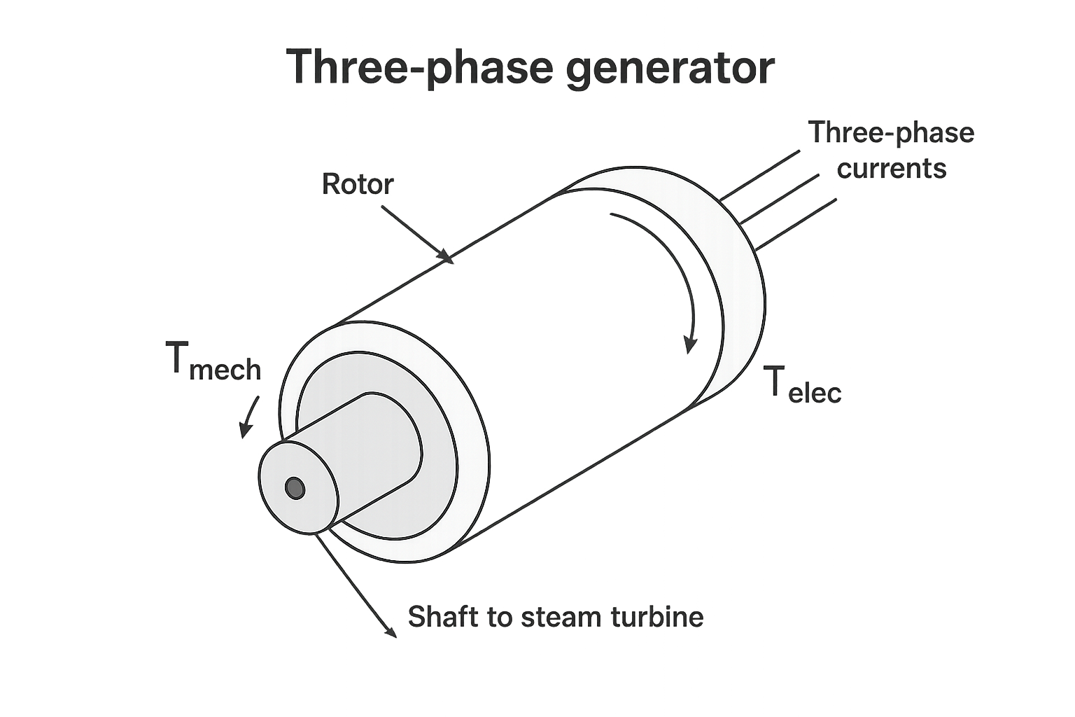
The dynamic interaction governing these opposing torque paths determines the net acceleration across the machine profile:

This interaction dictates three specific mechanical operational modes:

• Acceleration (Frequency Increases): Occurs when T_mech > T_elec. Input energy exceeds load consumption, causing the machine to speed up.
• Deceleration (Frequency Decreases): Occurs when T_mech < T_elec. Electrical demand outpaces turbine input, slowing the machine down.
• Steady Operation (Constant Frequency): Occurs when T_mech = T_elec. Power input matches power output, holding rotor speed perfectly constant.

5. Steady-State Frequency Control (Governor Control)

To preserve constant frequency under changing loads, mechanical input must adjust continuously. This regulation is handled automatically by a turbine speed governor.

If line frequency drops, the governor opens the valve to increase steam flow and boost generator output. If frequency rises, steam flow is restricted. Traditional systems track this via flywheel weights utilizing outward centrifugal force; modern setups use high-speed electronic sensors acting on the same core principle.

Governors are engineered with a dedicated droop characteristic. This means that as electrical load rises, the steady-state speed drops slightly (typically by about 4% from no-load to full 1.0 per-unit load rating).

The slope of this curve outlines the speed regulation of the turbine generator system. Adjusting internal spring tensions shifts the reference setting, moving the entire load-speed curve up or down while keeping its operating slope identical.

Why a perfectly flat characteristic is avoided: Constant-speed, horizontal zero-droop profiles make parallel operation highly unstable. Without a small drop in speed, governors lack a common feedback signal to detect balancing shifts, leading to highly volatile, uneven load distributions where one machine can dangerously overload while others under-load. A shared 4% droop ensures safe, cooperative load sharing across the grid.

6. Load Sharing Between Generators

Because all parallel-connected units are locked to the same electrical system, they must run at an identical system frequency. The distribution of the load across these units depends on their individual governor droop settings.

A generator with a steeper droop slope sheds load more quickly, while a unit with a flatter characteristic assumes a larger share of the demand. System operators tune reference points to distribute generation targets while holding network frequency stable.

7. Dynamic Regulation & Infinite Busbars

Dynamic Frequency Control: Speed governors do not react instantaneously; they feature a brief physical latency delay of around 0.3 seconds. During this initial window, the grid relies entirely on the stored rotational kinetic energy inside the spinning rotors. High system inertia helps reduce the rate of change of frequency (RoCoF) following large load events.

The Grid as an Infinite Busbar: Interconnected utility networks combine hundreds of large units, resulting in massive total inertia. Consequently, an isolated load change from a single asset has no noticeable impact on overall system frequency. The grid effectively behaves as an infinite busbar—acting as a stable voltage and frequency source that remains unchanged from the perspective of any individual machine.

Parallel Generator Worked Example